Iclass elite, continued

When I left off Elite iClasss hacking, the method of hacking iClass Elite was left a bit unfinished. Recently, another forum member reached out to me, gracefully lent me an elite-capable reader, an elite tag and a few standard tags, in order for me to be able to finish the work started. While key-extraction from the reader worked fine, actually dumping elite tags did not function properly. It turned out that part of the cipher implementation was wrong (technically, the hash1 implementation).

After that was fixed, I incorporated loclass into pm3 proper, and fixed up the dumper to be more stable. So, here’s how perform the reader-attack in two steps; first the OTA-attack, then the bruteforce:

Once that’s finished, you can dump a corresponding elite card:

You’ll notice that some bugs remain; the attack first misses one block, but it works the second time. Also, it reports “0 bytes dumped”, which is a flaw on the client side - nevertheless, the data is there on the screen. The next goal for iclass is to be able to do a full simulation; that is, not only simulate a UID, simulate a full tag loaded with data, similar to how hf mf eload <file> and hf mf sim works today.

Mifare revisited

And as we’re on the topic of Mifare. There’s been a long standing bug, where hf mf sim and hf mf sniff did not function properly. A couple of weeks back, myself and forum user piwi started investigating that. There were a couple of issues:

• The Miller decoder required far too long betweeen tag EOT and reader SOT.
• The built-in field detection was wrong, resulting in reader-field not being detected as active by the pm3 when doing tag simulations.
• An extra bit was sent OTA when simulating tags. This is both ‘wrong’ and costs ~20us.

See below for more information about OTA measurements.

Signals and scopes

Earlier, I used a Rigol DS1074 oscilloscope to perform measurements. This was a bit of a hassle, since I wasn’t able to find a good triggering mechanism, nor was I able to perform a long enough recording to be able to capture the specific data exchange that I was looking for; in practice I just froze the DSO at random and hoped for the best. This way, I was still able to capture data with a bit of luck:

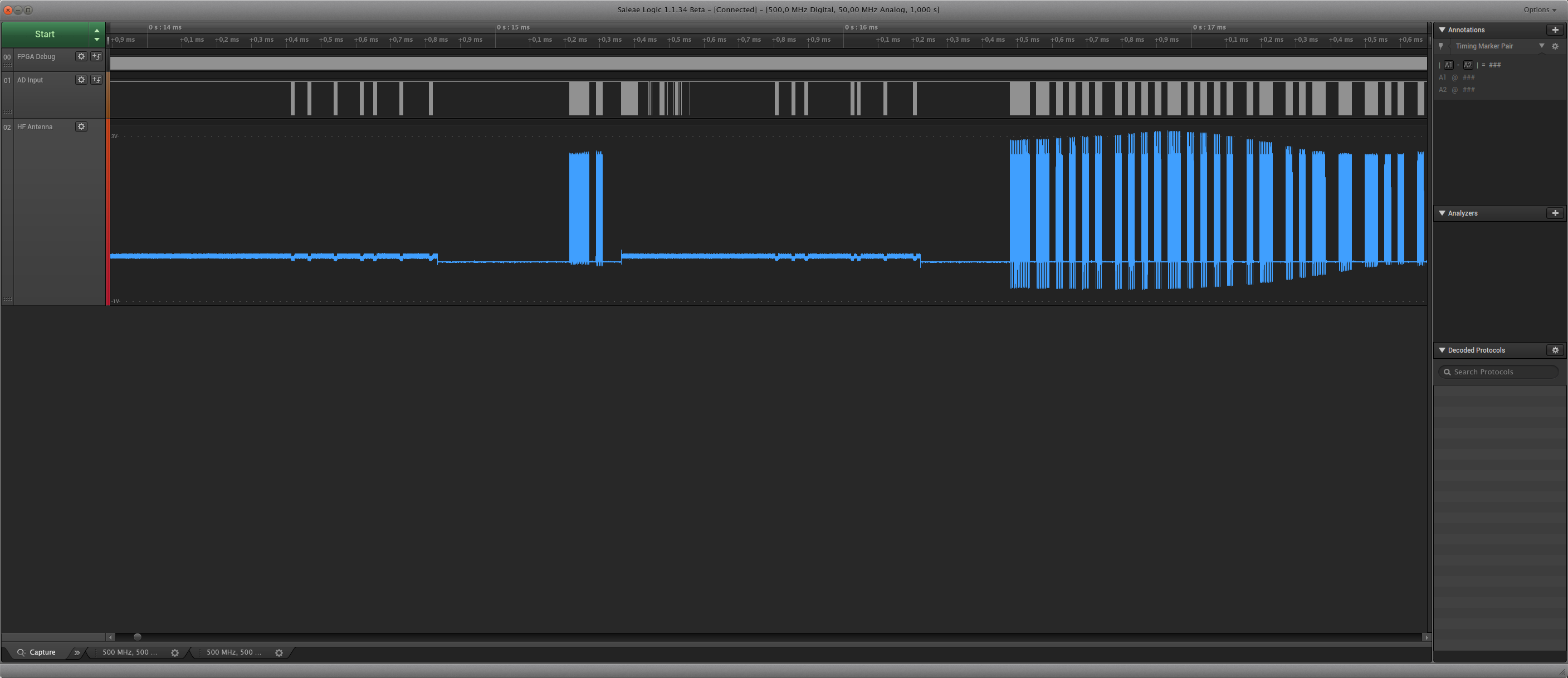
However, I recently got a Saleae Logic Pro 8, and decided to use this for investigating both iclass and the mifare issues. It’s a small logic analyzer which also has analog capture capabilties, being able to double as an oscilloscope. I’ve really come to adore the little thing; since it streams captured data over USB 3, it can capture as much as your ram can hold, allowing for several seconds of captures at 50 MSPS. This makes it trivial to capture a communication sequence and investigate exactly what it is you’re interested in.

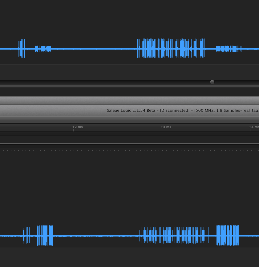
Here are some examples of traces captured with the Saleae. The upper one is simulation, the lower one is snoop of a regular tag. Both at the first tag response:

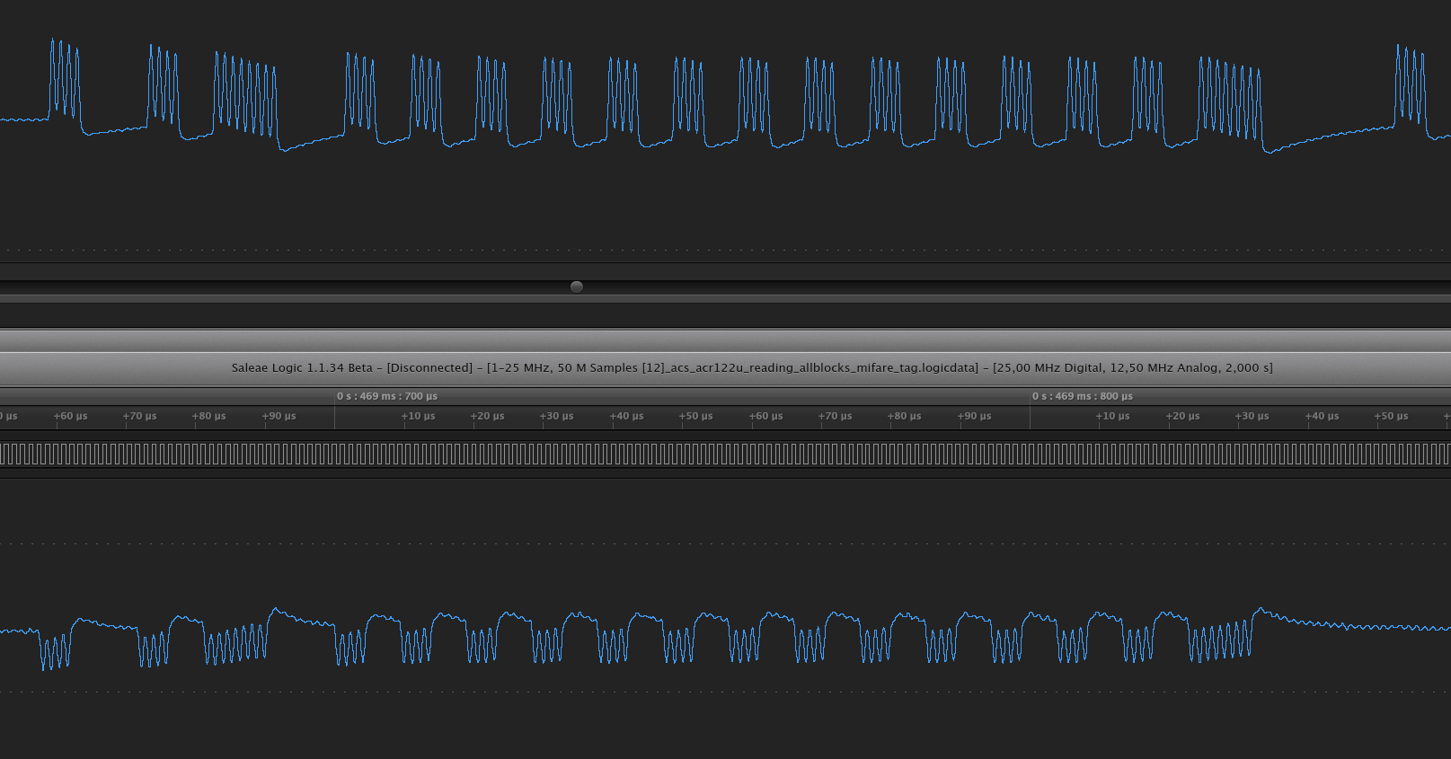
The extra bit sent during simulation is seen on the upper right side.

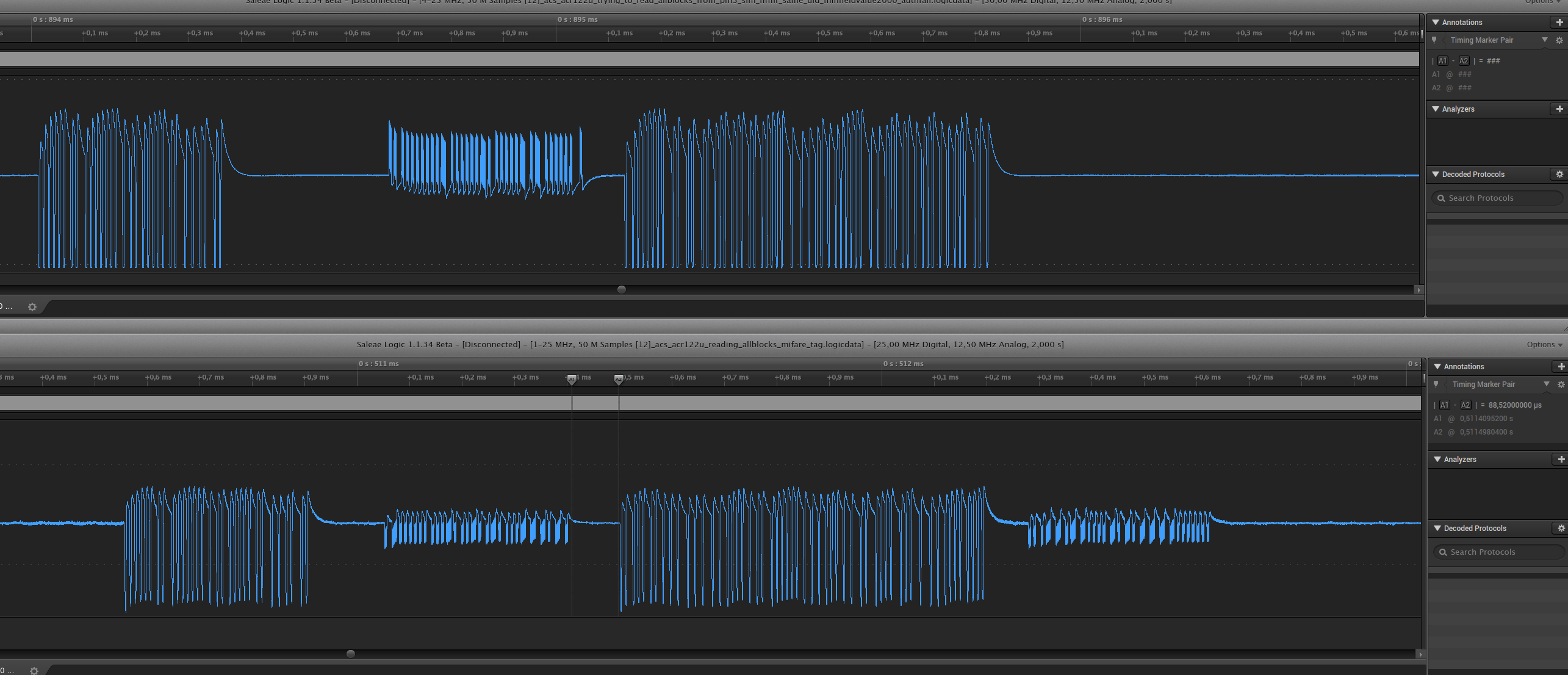
Below, the simulated tag fails to respond to a reader-command (the lower one is a proper tag):

Measuring OTA communications can be done in several ways.

1. Using probes on the PM3 antenna. This is what I did earlier. The drawback is that the signals are much stronger when the pm3 is active than passive. This is ok if you want to study how the pm3 signal looks, but less good if you want to compare a pm3 with a real tag.
2. Using probe on the AD input. The AD measures the voltage on the antenna. This requires the pm3 to been powered-on, as opposed to antenna-measurements. The readings above are both done on AD input.
3. Using a separate antenna probe. This is good since the readings do not depend on the PM3, which makes it very easy to compare a real tag to a simulated tag.

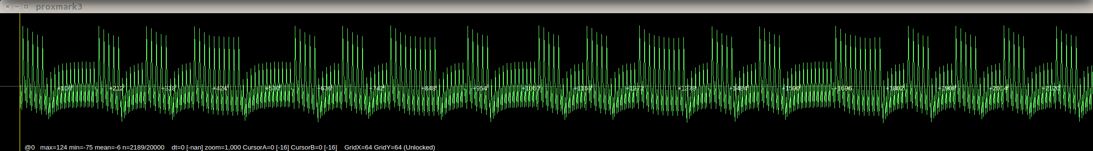
An example of using a probe directly on the HF antenna is below. As can be seen, it clearly ‘exaggarates’ the local (tag) signal, showing them as very strong, while the reader commands are captured as very tiny notches in comparison. :

In order to perform the third type of reading, it’s easy to manufacture a simple HF antenna with a piece of wire. I used 3 loops of wire, wound rectangularly a bit smaller than a credit card, and connected to the DSO. The image below is made using a separate snoop-antenna:

The Saleae device does some kind of interpolation, I believe that’s why the carrier frequency isn’t shown at all. However, that can be turned off for a more true representation of the signal OTA. Below are a couple of comparisons of the signal generated between an iclass reader and tag.

First, a zoomed out view where you can see the reader activating the 13.56MHz carrier field, and the ensuing communication. The peaks are reader modulations, the tag modulations cannot be seen here:

For comparison, the ‘Upsampled Pipeline’ version does not display the activation of the carrier:

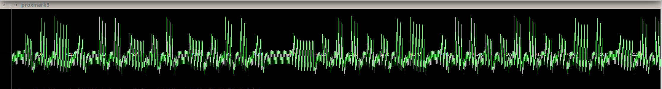
The same capture, but with more zoom. The tag modulations can be seen as small notches in the carrier:

While in the ‘Upsampled Pipeline’ version, the tag modulation is still not visible:

When doing these recordings, the placing of the antenna against the reader and the tag has large effects on the quality. In in these last measurements I just did to compare the different modes, I placed the antenna a bit haphazardly in relation to the reader and the tag; hence the extra-poor quality of the tag modulations. I recommend using rubber bands to affix the flimsy tags and antennas to the reader.

Anyway, the device is awesome, I really recommend it for geeking around with signals and and electronics.

Low frequency exploration

I then performed some more work on the LF-side of things. First off, support for longer sample recordings, both for lf read and lf snoop. It uses a configuration on the device side.

proxmark3> lf config
Usage: lf config [H|<divisor>] [b <bps>] [d <decim>] [a 0|1]          
Options:                  
       h             This help          
       L             Low frequency (125 KHz)          
       H             High frequency (134 KHz)          
       q <divisor>   Manually set divisor. 88-> 134KHz, 95-> 125 Hz          
       b <bps>       Sets resolution of bits per sample. Default (max): 8          
       d <decim>     Sets decimation. A value of N saves only 1 in N samples. Default: 1          
       a [0|1]       Averaging - if set, will average the stored sample value when decimating. Default: 1          
       t <threshold> Sets trigger threshold. 0 means no threshold          
Examples:          
      lf config b 8 L          
                    Samples at 125KHz, 8bps.          
      lf config H b 4 d 3          
                    Samples at 134KHz, averages three samples into one, stored with           
                    a resolution of 4 bits per sample.          
      lf read          
                    Performs a read (active field)          
      lf snoop          
                    Performs a snoop (no active field)  

The user can set the decimation and bits per sample. After read/snoop, the data is fetched as usual with data samples, which is alerted about the bps and thus unpacks it to normal 8-bit samples on the client-side. In order to run standard demodulators on it, you can then do (client side) un-decimation:

proxmark3> data undec h
Usage: data undec [factor]          
This function performs un-decimation, by repeating each sample N times          
Options:                  
       h            This help          
       factor       The number of times to repeat each sample.[default:2]          
Example: 'data undec 3'   

This affects also how lf read and lf snoop works, since they now don’t take any parameters. You just configure via lf config, then call read/snoop.

Example (no decimation):

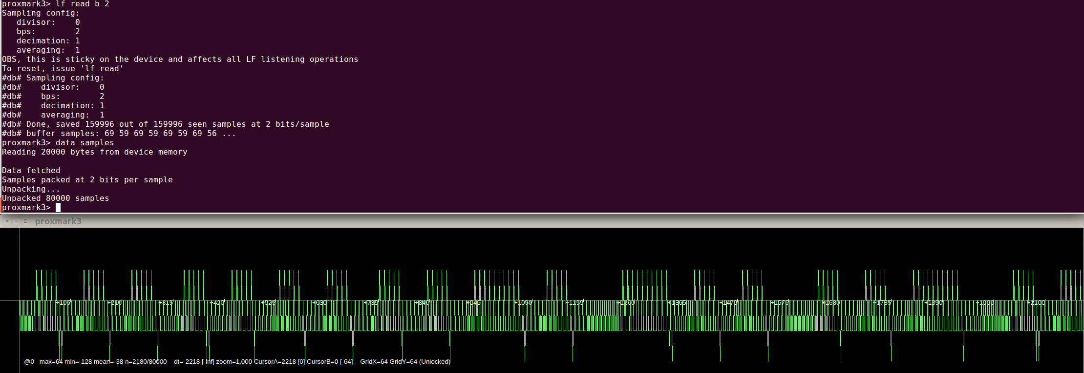
decimation by 2:

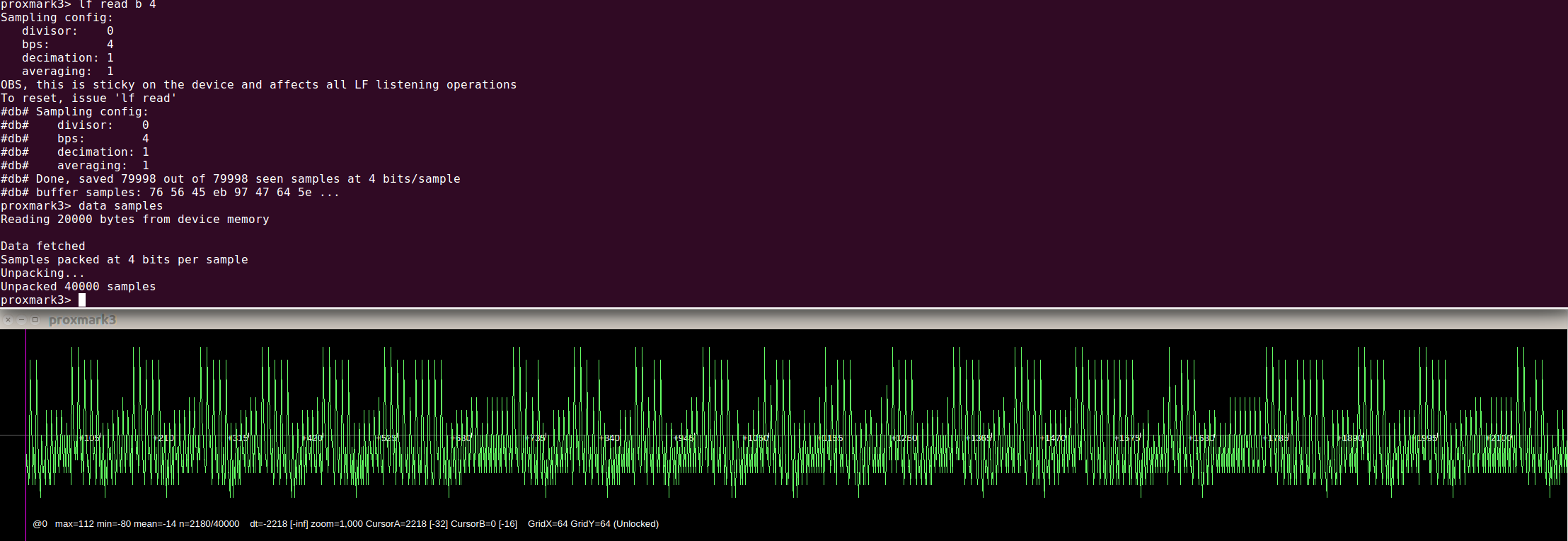
decimation by 4:

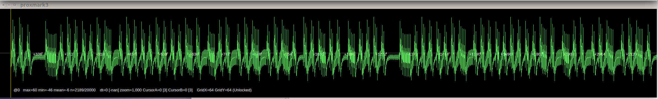
Signal with 4 bits per sample:

Signal with 2 bits per sample:

The effect of this is that the pm3 can now perform sampling of LF signals for several seconds, which may be useful in some scenarios.

Data plotting

The graphing functions in pm3 hasn’t been touched in a long time. Currently, I’m reworking that a tad. It’s been nagging me that when testing different modulations or clocks, the graph is ‘destroyed’. Effectively, this has been the workflow:

1. Load signal data load mysample
2. Graph signal data plot
3. Threshold data dirthreshold 10 -10
4. OOps, bad threshold. Go back to 1.

I decided to use two buffers instead, and have a knob to set the parameters; and provide instant feedback.

Here’s how it looks right now:

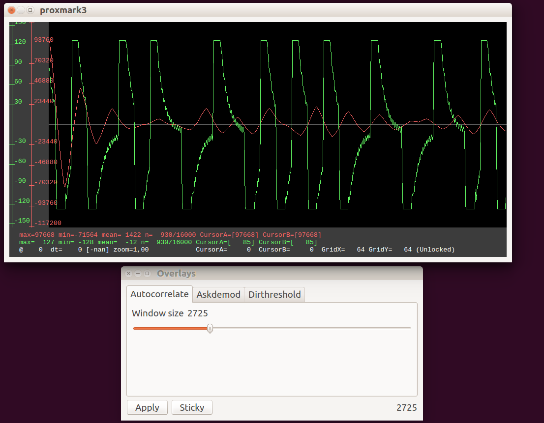
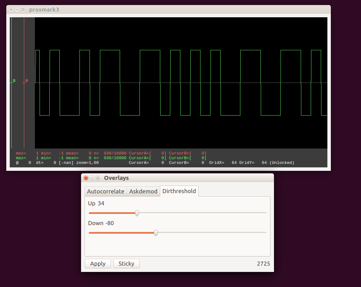
What you can’t see here, is that if you pull the slider to the left (increasing autocorrelatio ‘window’), the red graph updates in real time. The same thing with dirthreshold:

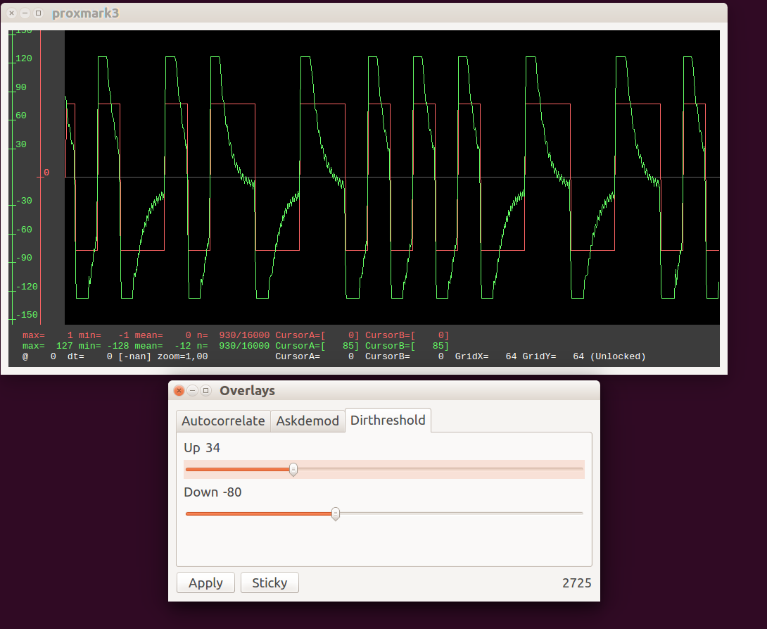
Once you’re happy with the settings, you can press apply, and the red signal is copied into the main signal buffer (graphbuffer):

This last part is still in a separate branch in github, and not part of the master code yet. We’ll see where it goes.

More features

There’s been a surge of PM3 development lately. Other members (marshmellow, iceman) have contributed major features in LF-area (new decoders for various types, new and improved demodulators) and scripting (identification/exploration of a common RFID-enabled toy), interaction with Mifare Desfire and Ultralight. It’s getting about time for a major version update soon.

2015-02-12

tweets

favorites